Data Visualization Makeover 04

Putting Visual Analytics into Practical Use

Author

Bryant Philippe Lee

Published

February 26, 2022

Objective

The objective is to uncover the impact of COVID-19 as well as the global economic and political dynamic in 2022 on Singapore bi-lateral trade (i.e. Import, Export and Trade Balance) by using appropriate analytical visualisation techniques to enhance user and data discovery experiences.

The visualization is created using the Merchandise Trade provided by Department of Statistics, Singapore (DOS).

Getting Started - Data Loading and Processing

Installing and loading the required libraries

pacman::p_load(scales, viridis, lubridate, ggthemes, gridExtra, tidyverse, readxl, knitr, data.table, readxl, lubridate, stringr, dplyr, gganimate, transformr, patchwork, countrycode)

Importing Data

This code chunk is to import the data from Merchandise Trade Excel File. The following sheets are within the file:

T1 = Import Data
T2 = Export Data

The data shows the import export relationship between Singapore and the other nations in terms of Million Dollar or Thousand Dollar

Data Structure

The Merchandise Trade data set is labeled with Thousand Dollars and Million Dollars. Further examination shows the following:

Million Dollars - Continent:

Listed under this category are continental data and values, as such are the summation of nations within these continents.
The summation of this continents (except for European Union as it is part of Europe) is = Total Merchandise Exports

Thousand Dollars - Nations:

Nation specific data and values

import_continent <- read_excel("data/Merchandise_Trade.xlsx", 
                          sheet = "T1",
                          range = cell_rows(10:16))%>%
  select(`Data Series`, contains(c("2019","2020", "2021", "2022"))) %>%
  slice(-1) %>%
  set_names(if_else(names(.) == "Data Series", "Country", names(.)))

import_continent$Country <- str_replace_all(import_continent$Country, "\\s*\\(.*?\\)", "")

import_continent

# A tibble: 5 × 49
  Country `2019 Dec` `2019 Nov` 2019 O…¹ 2019 …² 2019 …³ 2019 …⁴ 2019 …⁵ 2019 …⁶
  <chr>        <dbl>      <dbl>    <dbl>   <dbl>   <dbl>   <dbl>   <dbl>   <dbl>
1 America      5686.      6275.    5754.   5633.   6129.   5986.   5876.   5797.
2 Asia        27689.     27905    28378.  26350.  26672.  28473.  26052.  27541 
3 Europe       6315.      6827.    6625.   6310.   6534.   6325.   6055.   7987.
4 Oceania      1369.       841.     942.    867.   1015.    815.    504.    889.
5 Africa        521.       642      583.    290.    649.    430     493.    422.
# … with 40 more variables: `2019 Apr` <dbl>, `2019 Mar` <dbl>,
#   `2019 Feb` <dbl>, `2019 Jan` <dbl>, `2020 Dec` <dbl>, `2020 Nov` <dbl>,
#   `2020 Oct` <dbl>, `2020 Sep` <dbl>, `2020 Aug` <dbl>, `2020 Jul` <dbl>,
#   `2020 Jun` <dbl>, `2020 May` <dbl>, `2020 Apr` <dbl>, `2020 Mar` <dbl>,
#   `2020 Feb` <dbl>, `2020 Jan` <dbl>, `2021 Dec` <dbl>, `2021 Nov` <dbl>,
#   `2021 Oct` <dbl>, `2021 Sep` <dbl>, `2021 Aug` <dbl>, `2021 Jul` <dbl>,
#   `2021 Jun` <dbl>, `2021 May` <dbl>, `2021 Apr` <dbl>, `2021 Mar` <dbl>, …

export_continent <- read_excel("data/Merchandise_Trade.xlsx", 
                          sheet = "T2",
                          range = cell_rows(10:16))%>%
  select(`Data Series`, contains(c("2019","2020", "2021", "2022"))) %>%
  slice(-1) %>%
  set_names(if_else(names(.) == "Data Series", "Country", names(.)))

export_continent$Country <- str_replace_all(export_continent$Country, "\\s*\\(.*?\\)", "")

export_continent

# A tibble: 5 × 49
  Country `2019 Dec` `2019 Nov` 2019 O…¹ 2019 …² 2019 …³ 2019 …⁴ 2019 …⁵ 2019 …⁶
  <chr>        <dbl>      <dbl>    <dbl>   <dbl>   <dbl>   <dbl>   <dbl>   <dbl>
1 America      4614.      4822.    4938.   4754.   4838.   5209.   4990.   5809.
2 Asia        34177      34253.   33530.  32056.  33370.  32193.  29552.  32512.
3 Europe       3851       4173.    5163.   4007.   4278.   5232.   3891.   5480.
4 Oceania      1918.      2078.    2591.   2113.   2046    2022.   2118.   2070.
5 Africa        504.       432.     607.    563.    626.    735.    874.    761.
# … with 40 more variables: `2019 Apr` <dbl>, `2019 Mar` <dbl>,
#   `2019 Feb` <dbl>, `2019 Jan` <dbl>, `2020 Dec` <dbl>, `2020 Nov` <dbl>,
#   `2020 Oct` <dbl>, `2020 Sep` <dbl>, `2020 Aug` <dbl>, `2020 Jul` <dbl>,
#   `2020 Jun` <dbl>, `2020 May` <dbl>, `2020 Apr` <dbl>, `2020 Mar` <dbl>,
#   `2020 Feb` <dbl>, `2020 Jan` <dbl>, `2021 Dec` <dbl>, `2021 Nov` <dbl>,
#   `2021 Oct` <dbl>, `2021 Sep` <dbl>, `2021 Aug` <dbl>, `2021 Jul` <dbl>,
#   `2021 Jun` <dbl>, `2021 May` <dbl>, `2021 Apr` <dbl>, `2021 Mar` <dbl>, …

import_nation <- read_excel("data/Merchandise_Trade.xlsx", 
                          sheet = "T1",
                          range = cell_rows(10:129))%>%
  select(`Data Series`, contains(c("2019","2020", "2021", "2022"))) %>%
  slice(-c(1:7))%>%
  set_names(if_else(names(.) == "Data Series", "Country", names(.)))

import_nation$Country <- str_replace_all(import_nation$Country, "\\s*\\(.*?\\)", "")

import_nation

# A tibble: 112 × 49
   Country       2019 …¹ 2019 …² 2019 …³ 2019 …⁴ 2019 …⁵ 2019 …⁶ 2019 …⁷ 2019 …⁸
   <chr>           <dbl>   <dbl>   <dbl>   <dbl>   <dbl>   <dbl>   <dbl>   <dbl>
 1 Belgium        148564  112197  148895  109280  110542  140243  154637  220417
 2 Denmark         44062   53664  112559   59067   57022   53531   41769   89820
 3 France        1305861 1607039 1539927 1553172 1384504 1377160 1247644 1692436
 4 Germany, Fed… 1090801 1076037 1090588 1084790 1141855 1194530 1016793 1201604
 5 Greece          12161   14507    9397   12033   11920   12095   27007   12964
 6 Ireland         93080  111909   91189   72531   76235   93976   75391   79185
 7 Italy          547815  544113  499738  350214  451463  486021  420572  479798
 8 Luxembourg       2205   70742    4511    3546    3438    7249    9804    5269
 9 Netherlands    243929  382026  248639  262842  496961  298550  270901  510772
10 United Kingd… 1122876 1057533 1028921  961614 1044665  881698  852706  977237
# … with 102 more rows, 40 more variables: `2019 Apr` <dbl>, `2019 Mar` <dbl>,
#   `2019 Feb` <dbl>, `2019 Jan` <dbl>, `2020 Dec` <dbl>, `2020 Nov` <dbl>,
#   `2020 Oct` <dbl>, `2020 Sep` <dbl>, `2020 Aug` <dbl>, `2020 Jul` <dbl>,
#   `2020 Jun` <dbl>, `2020 May` <dbl>, `2020 Apr` <dbl>, `2020 Mar` <dbl>,
#   `2020 Feb` <dbl>, `2020 Jan` <dbl>, `2021 Dec` <dbl>, `2021 Nov` <dbl>,
#   `2021 Oct` <dbl>, `2021 Sep` <dbl>, `2021 Aug` <dbl>, `2021 Jul` <dbl>,
#   `2021 Jun` <dbl>, `2021 May` <dbl>, `2021 Apr` <dbl>, `2021 Mar` <dbl>, …

export_nation <- read_excel("data/Merchandise_Trade.xlsx", 
                          sheet = "T2",
                          range = cell_rows(10:101))%>%
  select(`Data Series`, contains(c("2019","2020", "2021", "2022"))) %>%
  slice(-c(1:7)) %>%
  set_names(if_else(names(.) == "Data Series", "Country", names(.)))

export_nation$Country <- str_replace_all(export_nation$Country, "\\s*\\(.*?\\)", "")

export_nation

# A tibble: 84 × 49
   Country       2019 …¹ 2019 …² 2019 …³ 2019 …⁴ 2019 …⁵ 2019 …⁶ 2019 …⁷ 2019 …⁸
   <chr>           <dbl>   <dbl>   <dbl>   <dbl>   <dbl>   <dbl>   <dbl>   <dbl>
 1 Belgium        498029  553449  635001  463503  338818  389853  318325 1380735
 2 Denmark         13039   11415   15446   12465   19571   21957   19587   27991
 3 France         415758  435599  429136  438494  429193  410138  360330  577736
 4 Germany, Fed…  601244  581154  718934  615005  637776  665181  596595  681759
 5 Greece          52483   89984  103260   70956   97643   99937  108931   99698
 6 Ireland         51855   37105   29955   18348   22930   48834   56440   46114
 7 Italy           60013   63034   75656   99466   75998   79456   76213  111059
 8 Luxembourg      12166   11691   10664    8097   15148   19069   13156   13103
 9 Netherlands    924561 1085006 1014106  761725  866614 1108801  934829 1110456
10 United Kingd…  371352  426137  805061  398734  683087  695876  351668  517108
# … with 74 more rows, 40 more variables: `2019 Apr` <dbl>, `2019 Mar` <dbl>,
#   `2019 Feb` <dbl>, `2019 Jan` <dbl>, `2020 Dec` <dbl>, `2020 Nov` <dbl>,
#   `2020 Oct` <dbl>, `2020 Sep` <dbl>, `2020 Aug` <dbl>, `2020 Jul` <dbl>,
#   `2020 Jun` <dbl>, `2020 May` <dbl>, `2020 Apr` <dbl>, `2020 Mar` <dbl>,
#   `2020 Feb` <dbl>, `2020 Jan` <dbl>, `2021 Dec` <dbl>, `2021 Nov` <dbl>,
#   `2021 Oct` <dbl>, `2021 Sep` <dbl>, `2021 Aug` <dbl>, `2021 Jul` <dbl>,
#   `2021 Jun` <dbl>, `2021 May` <dbl>, `2021 Apr` <dbl>, `2021 Mar` <dbl>, …

Exploring and Cleaning the Data

Pivoting Dataset

This section ensures that the datetime column labels are represented correctly. The dataset must be pivoted to reflect that.

imports_C_pivot <- import_continent %>%
  pivot_longer(
    cols = !"Country",
    names_to = "Month-Year",
    values_to = "Amount",
    values_drop_na = TRUE
  )

imports_C_pivot

# A tibble: 240 × 3
   Country `Month-Year` Amount
   <chr>   <chr>         <dbl>
 1 America 2019 Dec      5686.
 2 America 2019 Nov      6275.
 3 America 2019 Oct      5754.
 4 America 2019 Sep      5633.
 5 America 2019 Aug      6129.
 6 America 2019 Jul      5986.
 7 America 2019 Jun      5876.
 8 America 2019 May      5797.
 9 America 2019 Apr      6128 
10 America 2019 Mar      5529.
# … with 230 more rows

imports_N_pivot <- import_nation %>%
  pivot_longer(
    cols = !"Country",
    names_to = "Month-Year",
    values_to = "Amount",
    values_drop_na = TRUE
  )

imports_N_pivot

# A tibble: 5,376 × 3
   Country `Month-Year` Amount
   <chr>   <chr>         <dbl>
 1 Belgium 2019 Dec     148564
 2 Belgium 2019 Nov     112197
 3 Belgium 2019 Oct     148895
 4 Belgium 2019 Sep     109280
 5 Belgium 2019 Aug     110542
 6 Belgium 2019 Jul     140243
 7 Belgium 2019 Jun     154637
 8 Belgium 2019 May     220417
 9 Belgium 2019 Apr     134313
10 Belgium 2019 Mar     222413
# … with 5,366 more rows

exports_C_pivot <- export_continent %>%
  pivot_longer(
    cols = !"Country",
    names_to = "Month-Year",
    values_to = "Amount",
    values_drop_na = TRUE
  )

exports_C_pivot

# A tibble: 240 × 3
   Country `Month-Year` Amount
   <chr>   <chr>         <dbl>
 1 America 2019 Dec      4614.
 2 America 2019 Nov      4822.
 3 America 2019 Oct      4938.
 4 America 2019 Sep      4754.
 5 America 2019 Aug      4838.
 6 America 2019 Jul      5209.
 7 America 2019 Jun      4990.
 8 America 2019 May      5809.
 9 America 2019 Apr      5024.
10 America 2019 Mar      5281.
# … with 230 more rows

exports_N_pivot <- export_nation %>%
  pivot_longer(
    cols = !"Country",
    names_to = "Month-Year",
    values_to = "Amount",
    values_drop_na = TRUE
  )

exports_N_pivot

# A tibble: 4,032 × 3
   Country `Month-Year`  Amount
   <chr>   <chr>          <dbl>
 1 Belgium 2019 Dec      498029
 2 Belgium 2019 Nov      553449
 3 Belgium 2019 Oct      635001
 4 Belgium 2019 Sep      463503
 5 Belgium 2019 Aug      338818
 6 Belgium 2019 Jul      389853
 7 Belgium 2019 Jun      318325
 8 Belgium 2019 May     1380735
 9 Belgium 2019 Apr      277437
10 Belgium 2019 Mar      274500
# … with 4,022 more rows

Organizing Month-Year

This Section converts the “Month-Year” column to datetime.

imports_C_pivot$`Month-Year` <- as.Date(paste(imports_C_pivot$`Month-Year`, "01"), format = "%Y %b %d")

imports_C_pivot

# A tibble: 240 × 3
   Country `Month-Year` Amount
   <chr>   <date>        <dbl>
 1 America 2019-12-01    5686.
 2 America 2019-11-01    6275.
 3 America 2019-10-01    5754.
 4 America 2019-09-01    5633.
 5 America 2019-08-01    6129.
 6 America 2019-07-01    5986.
 7 America 2019-06-01    5876.
 8 America 2019-05-01    5797.
 9 America 2019-04-01    6128 
10 America 2019-03-01    5529.
# … with 230 more rows

imports_N_pivot$`Month-Year` <- as.Date(paste(imports_N_pivot$`Month-Year`, "01"), format = "%Y %b %d")

imports_N_pivot

# A tibble: 5,376 × 3
   Country `Month-Year` Amount
   <chr>   <date>        <dbl>
 1 Belgium 2019-12-01   148564
 2 Belgium 2019-11-01   112197
 3 Belgium 2019-10-01   148895
 4 Belgium 2019-09-01   109280
 5 Belgium 2019-08-01   110542
 6 Belgium 2019-07-01   140243
 7 Belgium 2019-06-01   154637
 8 Belgium 2019-05-01   220417
 9 Belgium 2019-04-01   134313
10 Belgium 2019-03-01   222413
# … with 5,366 more rows

exports_C_pivot$`Month-Year` <- as.Date(paste(exports_C_pivot$`Month-Year`, "01"), format = "%Y %b %d")

exports_C_pivot

# A tibble: 240 × 3
   Country `Month-Year` Amount
   <chr>   <date>        <dbl>
 1 America 2019-12-01    4614.
 2 America 2019-11-01    4822.
 3 America 2019-10-01    4938.
 4 America 2019-09-01    4754.
 5 America 2019-08-01    4838.
 6 America 2019-07-01    5209.
 7 America 2019-06-01    4990.
 8 America 2019-05-01    5809.
 9 America 2019-04-01    5024.
10 America 2019-03-01    5281.
# … with 230 more rows

exports_N_pivot$`Month-Year` <- as.Date(paste(exports_N_pivot$`Month-Year`, "01"), format = "%Y %b %d")

exports_N_pivot

# A tibble: 4,032 × 3
   Country `Month-Year`  Amount
   <chr>   <date>         <dbl>
 1 Belgium 2019-12-01    498029
 2 Belgium 2019-11-01    553449
 3 Belgium 2019-10-01    635001
 4 Belgium 2019-09-01    463503
 5 Belgium 2019-08-01    338818
 6 Belgium 2019-07-01    389853
 7 Belgium 2019-06-01    318325
 8 Belgium 2019-05-01   1380735
 9 Belgium 2019-04-01    277437
10 Belgium 2019-03-01    274500
# … with 4,022 more rows

Merge Dataset for both Continental and National Values

This section creates the consolidated dataset for both continental and national datasets with the following improvements:

Net Trade = Exports - Imports
Omit of all NA values

continent <- merge(x=imports_C_pivot , y=exports_C_pivot, by= c("Country", "Month-Year"), all.x = TRUE, all.y = TRUE)

Net_Trade = continent$Amount.y - continent$Amount.x

continent$Net_Trade <- Net_Trade

na.omit(continent) %>%
  rename(
    Continent = Country,
    Date = `Month-Year`,
    Imports = Amount.x,
    Exports = Amount.y
  )

nation <- merge(x=imports_N_pivot , y=exports_N_pivot, by= c("Country", "Month-Year"), all.x = TRUE, all.y = TRUE)

Net_Trade = nation$Amount.y - nation$Amount.x

nation$Net_Trade <- Net_Trade

na.omit(nation) %>%
  rename(
    Date = `Month-Year`,
    Imports = Amount.x,
    Exports = Amount.y
  )

Continental Trade Analysis - Visual Exploration

This section explores macro trade relationship of Singapore on the continental level.

Line Graph Visualization for Imports and Exports

Code

continent_import <- ggplot(continent,
       aes(x = `Month-Year`, y = Amount.x, color = Country)) +
  geom_line()+
  labs (x = "Date",
        y = "Import in Million Dollars",
        fill = "Continent",
        title = "Import in Million Dollars by Continent") +
  scale_x_date(date_labels = "%b-%y")+
  theme_bw() 

continent_export <- ggplot(continent,
       aes(x = `Month-Year`, y = Amount.y, color = Country)) +
  geom_line()+
  labs (x = "Date",
        y = "Export in Million Dollars",
        fill = "Continent",
        title = "Export in Million Dollars by Continent") +
  scale_x_date(date_labels = "%b-%y")+
  theme_bw()

continent_import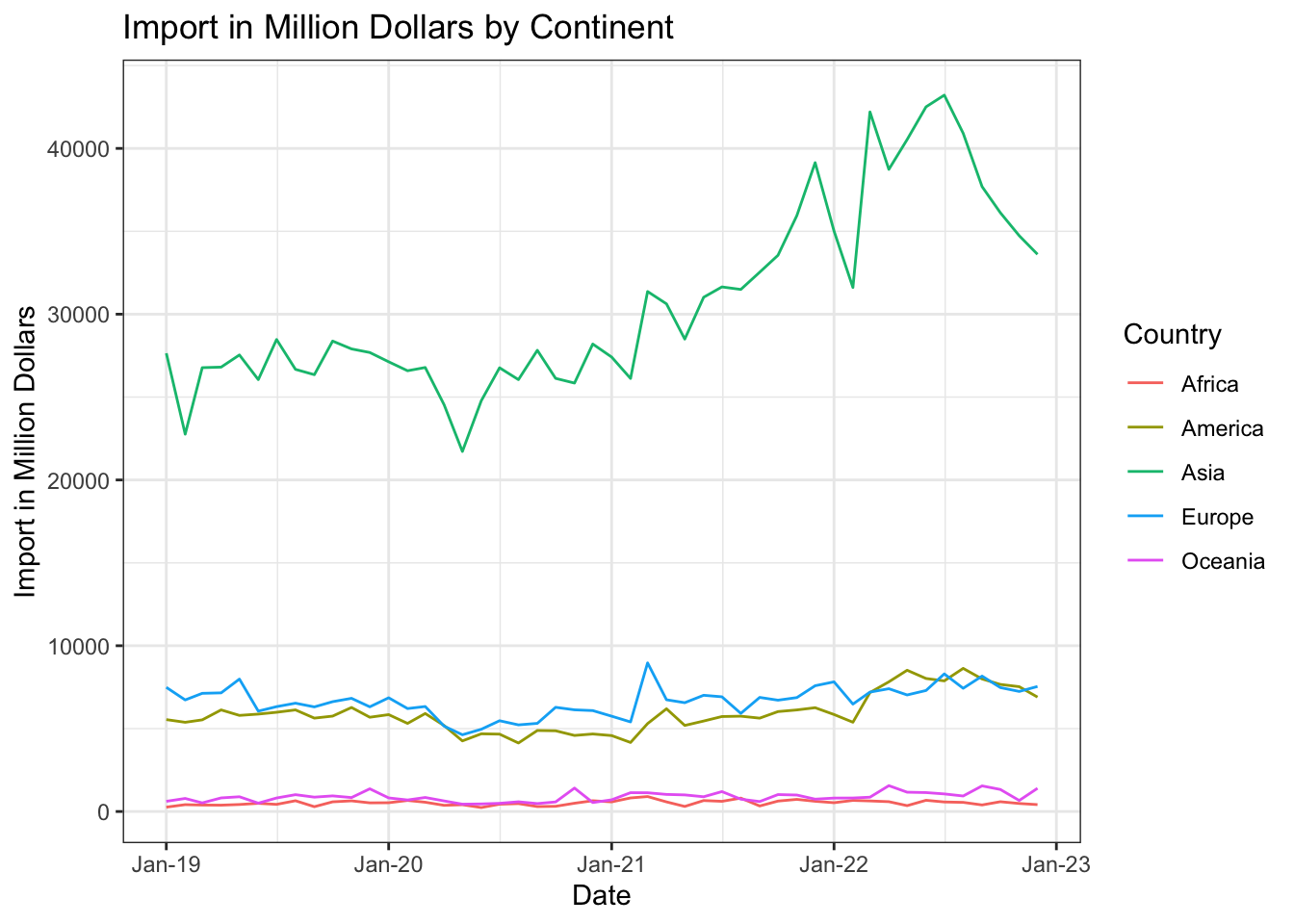

continent_export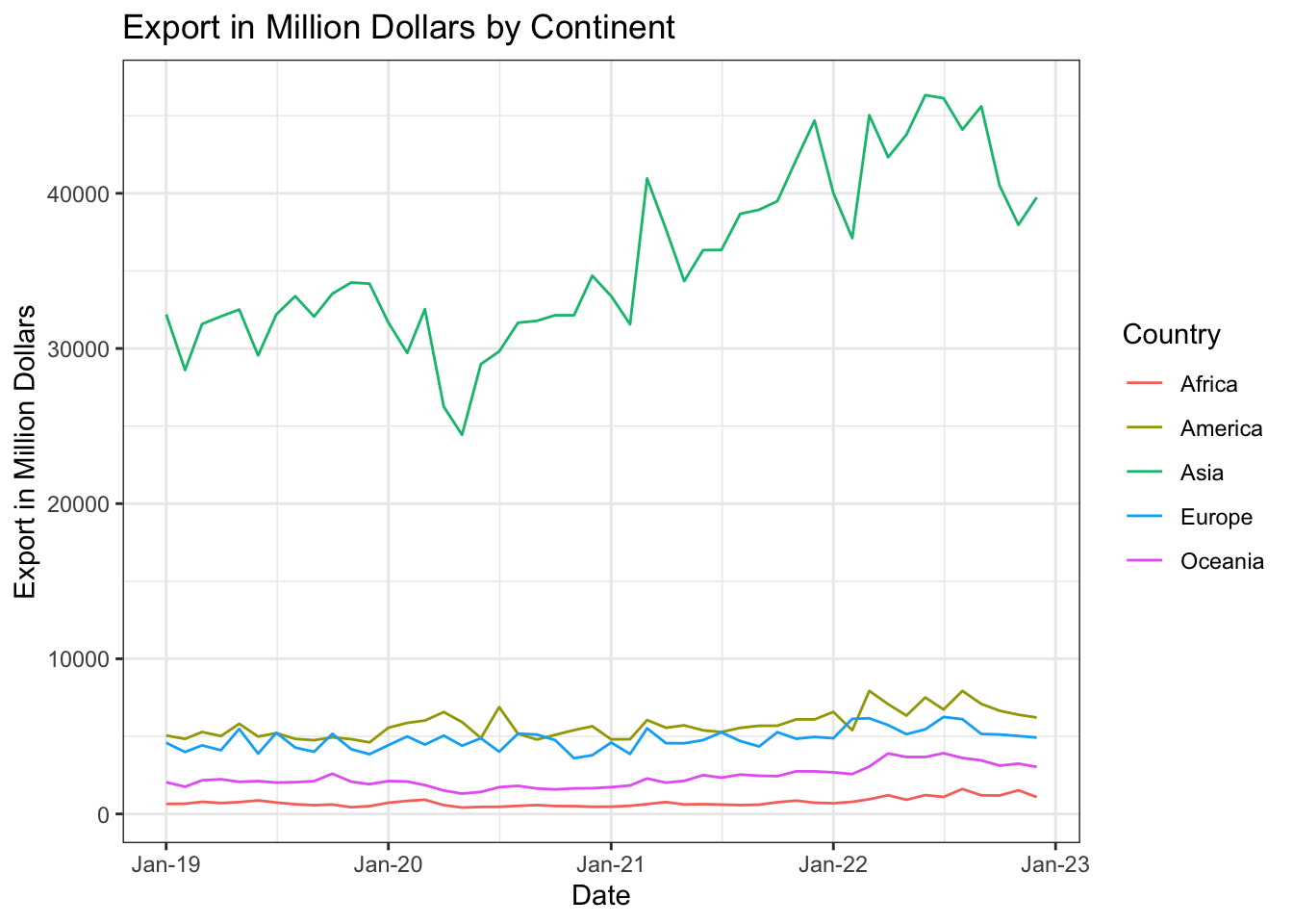

A simple beginning in visual analysis is a line chart to see the time series impact on both imports and exports. Here is the following insights:

Asia remains as the highest import export partner for Singapore. Consistently, from 2019 to 2022, Asia remains as the top import export partner of Singapore due to proximity. America and Europe follows as close 2nd and 3rd.
COVID 19 had none to minimal impact to Singapore’s Macro Trade Relationship. Year 2019 and 2020 - 2021 show no distinct drop in import and export amount (drop = significant change in numbers as minimal up and downs are expected).

Animated Time Series Scatter Plot

Code

ggplot(continent, aes(x = Amount.x, y = Amount.y, size = Net_Trade, color = Country)) + 
  geom_point(show.legend = FALSE, alpha = 0.7) +
  scale_color_viridis_d() +
  scale_size(range = c(2, 12)) +
  transition_time(continent$`Month-Year`) +
  labs(title = "Animated Scatterplot per Continent per Year: {frame_time}", x = "Imports", y = "Exports", fill = "Continent") +
  theme(legend.position = "bottom") + 
  theme_bw() + 
  facet_wrap(~Country)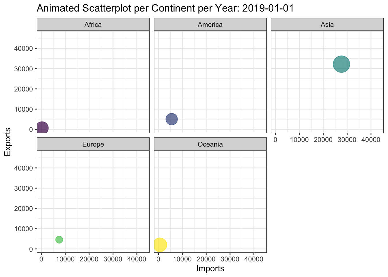

The Animated Scatter plot refocuses that Asia is the highest import export trade partner for Singapore, though there is an additional insight

Asia remains as the highest import export partner and moving to 2022, both import and export increases as it reaches 2022 as the other continent remained constant.
Europe shows periods of fluctuations in the index (export/import) as compared to the more stable continents.

Next Step

Visualize and Analyze nations within Asia and Europe separately to check and describe the time series progress of the import export trade amount.

Asian Trade Analysis - Visual Exploration

This section explores the macro economic trade relation of Singapore to its Asian Trade partners.

Identifying Country - Continent Labels

This section adds a continent label to the nation database identifying which continent a country belongs to.

countrycode() Package

You can use the countrycode() package to identify the continent and region of the country

continent = Continent as defined in the World Bank Development Indicators
un.regionsub.name: United Nations sub-region name

nation$Continent <- countrycode(sourcevar = nation$Country,
                            origin = "country.name",
                            destination = "continent")

Warning in countrycode_convert(sourcevar = sourcevar, origin = origin, destination = dest, : Some values were not matched unambiguously: Cocos Islands, Commonwealth Of Independent States, French Southern Territories, Micronesia, Other Countries In America, Other Countries In Oceania, Yemen Democratic

nation$Continent[nation$Country == "Other Country"] <- "Unknown"

nation$Region <- countrycode(sourcevar = nation$Country,
                            origin = "country.name",
                            destination = "un.regionsub.name")

Warning in countrycode_convert(sourcevar = sourcevar, origin = origin, destination = dest, : Some values were not matched unambiguously: Commonwealth Of Independent States, Micronesia, Netherlands Antilles, Other Countries In America, Other Countries In Oceania, Taiwan, Yemen Democratic

nation$Region[nation$Country == "Other Country"] <- "Unknown"

nation <- na.omit(nation)

nation

nation_asia <- nation %>%
  filter(str_detect(Continent, "Asia")) %>%
  select(-(Continent))

nation_asia

nation_eu <- nation %>%
  filter(str_detect(Continent, "Europe")) %>%
  select(-(Continent))

nation_eu

Asia Sub Region Visualization

Code

ggplot(nation_asia, aes(x = Amount.x, y = Amount.y, size = Net_Trade, color = Country)) + 
  geom_point(show.legend = FALSE, alpha = 0.7) +
  scale_color_viridis_d() +
  scale_size(range = c(2, 12)) +
  transition_time(nation_asia$`Month-Year`) +
  labs(title = "Animated Scatterplot per Asian Region per Year: {frame_time}", x = "Imports", y = "Exports", fill = "Region") +
  theme(legend.position = "bottom") + 
  theme_bw() + 
  facet_wrap(~Region)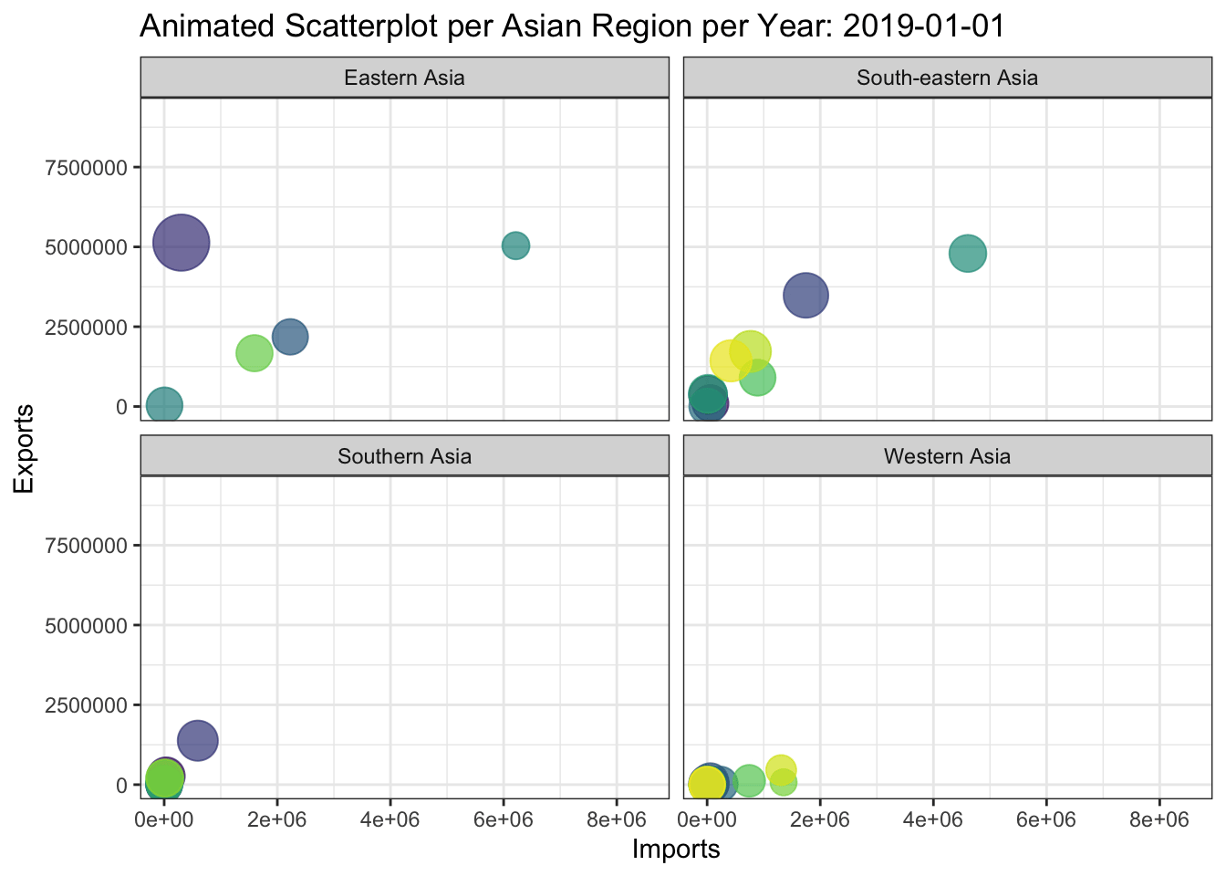

Based on the Animated Scatter Plot, the following insights are:

East Asia shows high import and export contribution. It is noted that there is a nation that have seen fluctuations in positioning in 2021 - 2022
Southeast Asia shows a more stable amount, thoigh there is a nation with more fluctuating position

East Asian Import Export Visualization

This section shows the trade relation in East Asia.

Code

nation_asia_ea <- nation_asia %>%
  filter(str_detect(Region, "Eastern Asia")) %>%
  select(-(Region))


asia_ea_import <- ggplot(nation_asia_ea,
       aes(x = `Month-Year`, y = Amount.x, color = Country)) +
  geom_line()+
  labs (x = "Date",
        y = "Import in Thousand Dollars",
        fill = "Country",
        title = "Import in Thousand Dollars by east Asian Country") +
  scale_x_date(date_labels = "%b-%y")+
  theme_bw() 

asia_ea_export <- ggplot(nation_asia_ea,
       aes(x = `Month-Year`, y = Amount.y, color = Country)) +
  geom_line()+
  labs (x = "Date",
        y = "Export in Thousand Dollars",
        fill = "Country",
        title = "Export in Thousand Dollars by East Asian Country") +
  scale_x_date(date_labels = "%b-%y")+
  theme_bw()

Code

asia_ea_import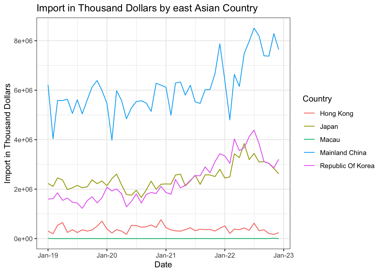

Code

asia_ea_export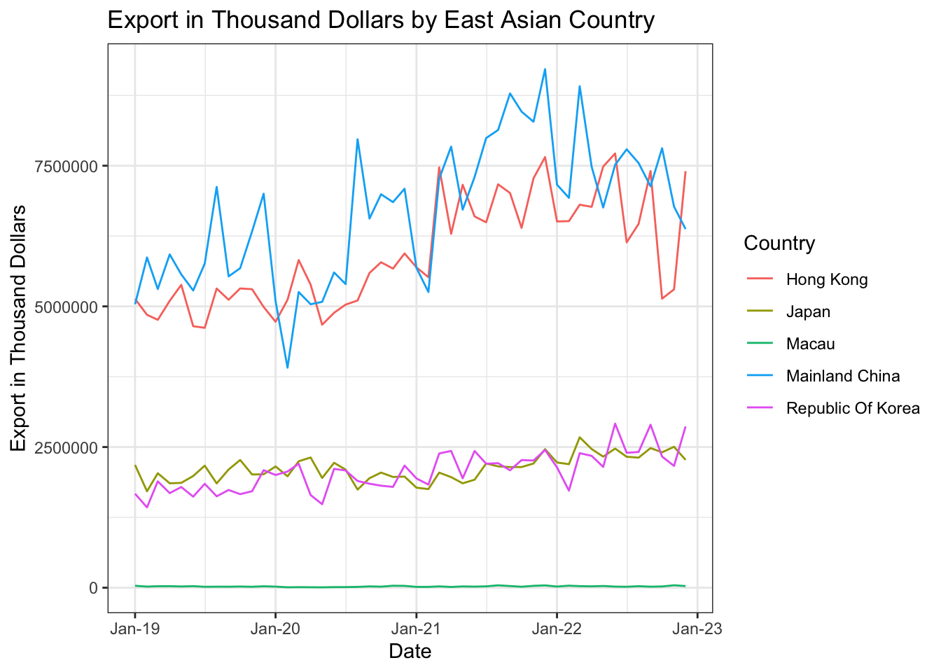

Code

ggplot(nation_asia_ea,
  aes(x = `Month-Year`, y = Amount.x, color = Country)) +
  geom_line() +
  scale_color_viridis_d() +
  labs(x = "Date",
       y = "Net Trade",
       fill = "Country",
       title = "Net Trade by East Asian Country") +
  theme(legend.position = "top") +
  theme_bw() +
  geom_point() +
  transition_reveal(nation_asia_ea$`Month-Year`)

`geom_line()`: Each group consists of only one observation.
ℹ Do you need to adjust the group aesthetic?
`geom_line()`: Each group consists of only one observation.
ℹ Do you need to adjust the group aesthetic?

Insights on the East Asian Region

Singapore has the highest Import and Export Trade relationship with Mainland China. This is due to being supported by the updated bilateral agreement made in 2019. Given Singapore is one of the biggest trade hubs and China as a manufacturing hub, Merchandise Trade between these nations are part of the supply chain such as electronic equipment, machinery and minerals.

Singapore - China Net Trade is higher in favor of Singapore (higher export). This is due to Singapore exporting more variety of goods from consumer to manufacturing requirements to China.

Singapore - China Trade Relationship

SINGAPORE-CHINA

In 2020, Singapore exported $42.9B to China. The main products that Singapore exported to China are Integrated Circuits ($10.6B), Ethylene Polymers ($2.25B), and Machinery Having Individual Functions ($1.86B).

CHINA-SINGAPORE

In 2020, China exported $54B to Singapore. The main products that China exported to Singapore were Integrated Circuits ($5.55B), Refined Petroleum ($4.88B), and Broadcasting Equipment ($3.97B). South East Asian Import Export Visualization

Singapore also have a high export low import relationship with Hong Kong. This is due to Hong Kong primarily acting as Financial Services Sector with minimal merchandise export on its own and rely on imports for consumer goods.

South East Asian Import Export Visualization

This section shows the trade relation in South East Asia.

Code

nation_asia_sea <- nation_asia %>%
  filter(str_detect(Region, "South-eastern Asia")) %>%
  select(-(Region))


asia_sea_import <- ggplot(nation_asia_sea,
       aes(x = `Month-Year`, y = Amount.x, color = Country)) +
  geom_line()+
  labs (x = "Date",
        y = "Import in Thousand Dollars",
        fill = "Country",
        title = "Import in Thousand Dollars by Southeast Asian Country") +
  scale_x_date(date_labels = "%b-%y")+
  theme_bw() 

asia_sea_export <- ggplot(nation_asia_sea,
       aes(x = `Month-Year`, y = Amount.y, color = Country)) +
  geom_line()+
  labs (x = "Date",
        y = "Export in Thousand Dollars",
        fill = "Country",
        title = "Export in Thousand Dollars by Southeast Asian Country") +
  scale_x_date(date_labels = "%b-%y")+
  theme_bw()

asia_sea_import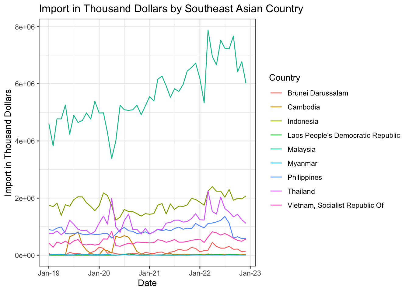

asia_sea_export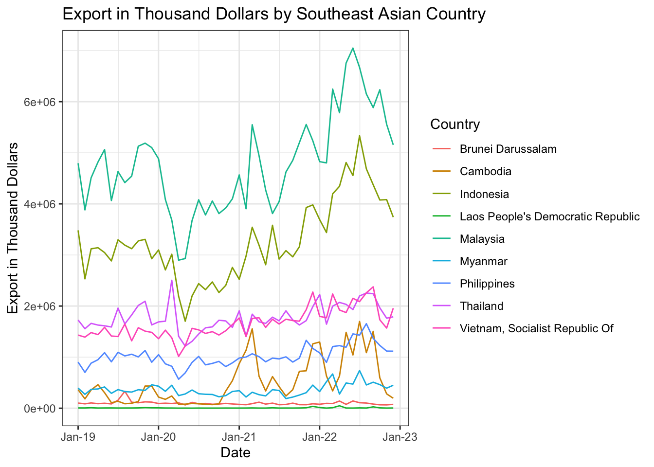

Code

ggplot(nation_asia_sea,
  aes(x = `Month-Year`, y = Amount.x, color = Country)) +
  geom_line() +
  scale_color_viridis_d() +
  labs(x = "Date",
       y = "Net Trade",
       fill = "Country",
       title = "Net Trade by Southeast Asian Country") +
  theme(legend.position = "top") +
  theme_bw() +
  geom_point() +
  transition_reveal(nation_asia_sea$`Month-Year`)

`geom_line()`: Each group consists of only one observation.
ℹ Do you need to adjust the group aesthetic?
`geom_line()`: Each group consists of only one observation.
ℹ Do you need to adjust the group aesthetic?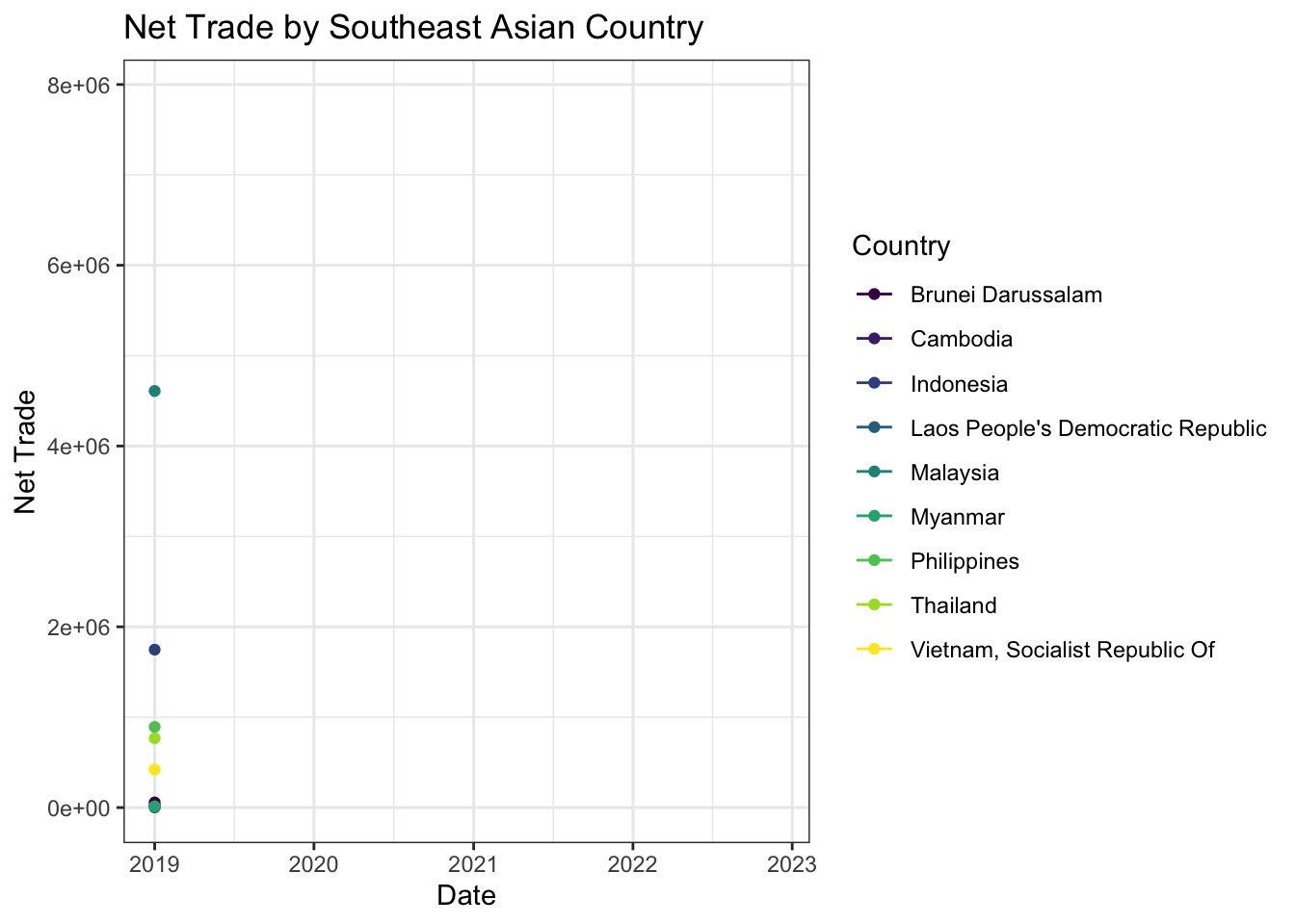

Insights on the South East Asian Region

Malaysia is the top import and export trade partner with Singapore. This is due to proximity between the nations. Furthermore. Net Trade has higher export with Singapore

Singapore - Malaysia Trade Relationship

MALAYSIA-SINGAPORE

In 2020, Malaysia exported $36.5B to Singapore. The main products that Malaysia exported to Singapore are Integrated Circuits ($11.1B), Refined Petroleum ($5.63B), and Office Machine Parts ($1.24B).

SINGAPORE-MALAYSIA

In 2020, Singapore exported $22.9B to Malaysia. The main products that Singapore exported to Malaysia were Integrated Circuits ($5.7B), Refined Petroleum ($4.33B), and Gold ($894M).

Singapore has a high export to Indonesia due to the high amounts of Gold and manufacturing parts sent over. Similar to nations that Singapore does bilateral trades of similar good, higher exports are primarily due to higher variety of goods.

European Trade Analysis - Visual Exploration

This section explores the macro economic trade relation of Singapore to its European Trade partners.

Europe Sub Region Visualization

Code

ggplot(nation_eu, aes(x = Amount.x, y = Amount.y, size = Net_Trade, color = Country)) + 
  geom_point(show.legend = FALSE, alpha = 0.7) +
  scale_color_viridis_d() +
  scale_size(range = c(2, 12)) +
  transition_time(nation_eu$`Month-Year`) +
  labs(title = "Animated Scatterplot per European Region per Year: {frame_time}", x = "Imports", y = "Exports", fill = "Region") +
  theme(legend.position = "bottom") + 
  theme_bw() + 
  facet_wrap(~Region)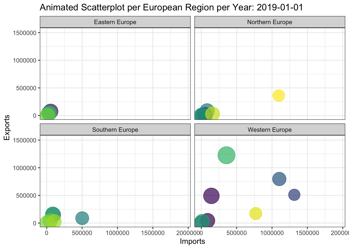

Based on the animated scatter plot, Western European nations have more dynamic trade relations as compared to others

Western European Import Export Visualization

This section shows the trade relation in West Europe.

Code

nation_eu_west <- nation_eu %>%
  filter(str_detect(Region, "Western Europe")) %>%
  select(-(Region))


eu_west_import <- ggplot(nation_eu_west,
       aes(x = `Month-Year`, y = Amount.x, color = Country)) +
  geom_line()+
  labs (x = "Date",
        y = "Import in Thousand Dollars",
        fill = "Country",
        title = "Import in Thousand Dollars by West Euro Country") +
  scale_x_date(date_labels = "%b-%y")+
  theme_bw() 

eu_west_export <- ggplot(nation_eu_west,
       aes(x = `Month-Year`, y = Amount.y, color = Country)) +
  geom_line()+
  labs (x = "Date",
        y = "Export in Thousand Dollars",
        fill = "Country",
        title = "Export in Thousand Dollars by West Euro Country") +
  scale_x_date(date_labels = "%b-%y")+
  theme_bw()

eu_west_import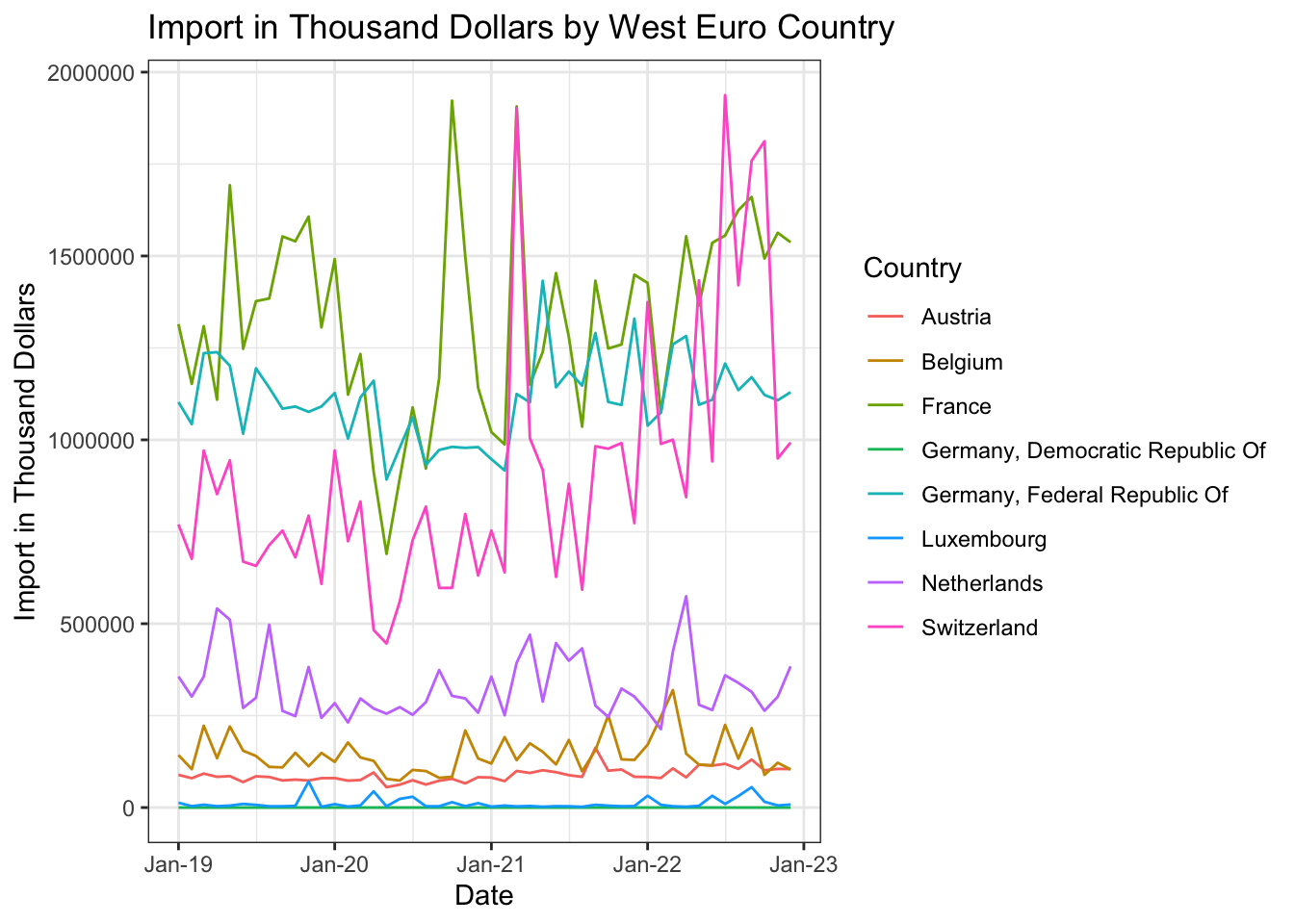

eu_west_import

Code

ggplot(nation_eu_west,
  aes(x = `Month-Year`, y = Amount.x, color = Country)) +
  geom_line() +
  scale_color_viridis_d() +
  labs(x = "Date",
       y = "Net Trade",
       fill = "Country",
       title = "Net Trade by West Euro Country") +
  theme(legend.position = "top") +
  theme_bw() +
  geom_point() +
  transition_reveal(nation_eu_west$`Month-Year`)

`geom_line()`: Each group consists of only one observation.
ℹ Do you need to adjust the group aesthetic?
`geom_line()`: Each group consists of only one observation.
ℹ Do you need to adjust the group aesthetic?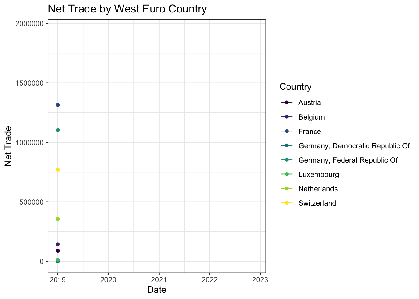

Insights on the Western European Region

As compared to Asian Trade partners, Western Europe experience high levels of fluctuation, presenting no clear front runner in trade relations with Singapore. This may be due to West Europe being majority part of the European Union and its ‘Single Market’. The ‘Single Market’ allows companies in Europe to operate in all nation states and be able to cooperatively export their products as a block while import products outside in bulk as well.